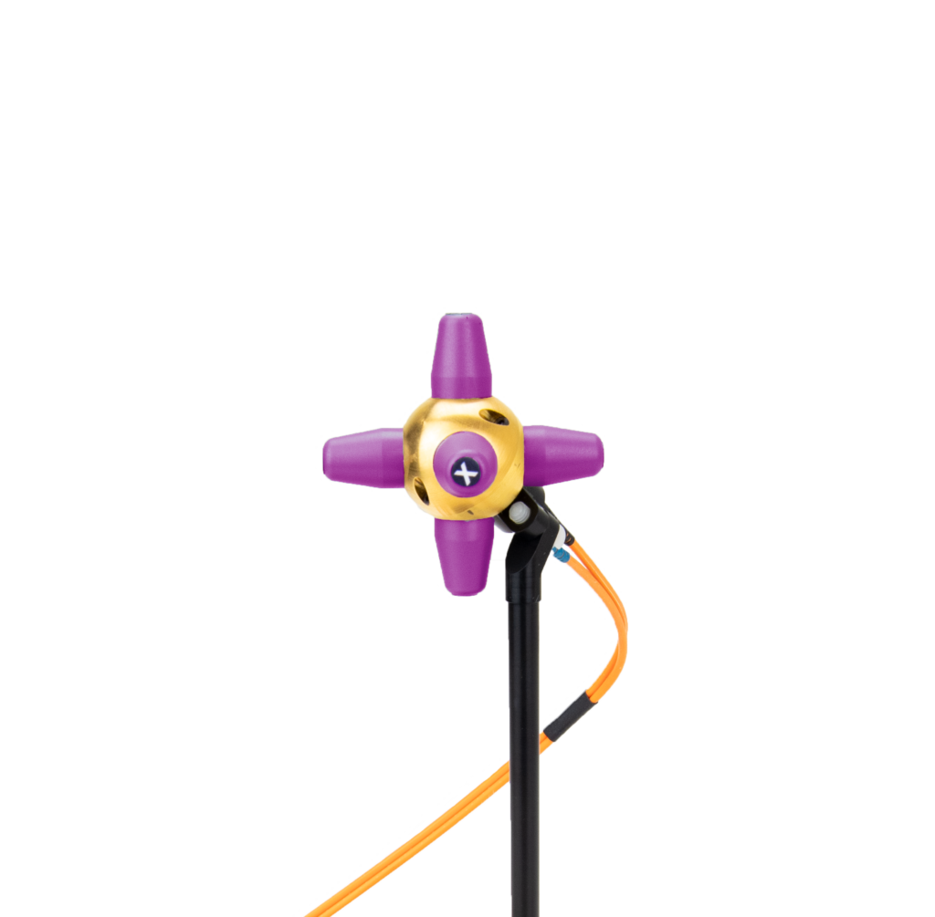
Measuring isotropic field strength
Isotropic Electric field probes generally make use of 3 antennae, orientated in the X-, Y and Z direction. The effective field strength measured is determined by the following calculation. The root mean square of the sum of the measured values of the 3 axis or in short:
E [V/m] = (Ex^2 + Ey^2 + Ez^2) ^0.5
Some probes determine the isotropic value by combining the amplitudes for the all axis in an electronic way. Before the amplitude is measured by the measurement circuit inside the probe. These probes are not able to display the field strength different field direction separately. They can only display the isotropic field strength. The disadvantage of this method is that it is not possible to apply correction values to the independent axis. This results in a higher measurement uncertainty.
A better way to combine the signals for the 3 axis is done by measuring the three axis independently. Probe which are capable of this will be able to display the field strength for the X, Y and Z direction independently. Not only that be these probes are capable to use this data to calculate the isotropic value. In this case, correction factors can be measured and applied to each axis separately resulting in the highest accuracy.
Probe Calibration.
When a field probe is calibrated, a known field strength is generated in one field direction (for example in vertical direction). The probe (EUT) is positioned in this known field, with one axis in parallel to the generated field.This calibration procedure is repeated with the X, Y and Z axis of the probe parallel to the field respectively.For each axis (and each calibration frequency), the correction factor is linear expressed and calculated by:
Kx,y,z (lin) = Egenerated / Emeasured
The above method will result in a correction factor per axis. The correction factor can also be expressed logarithmic (in dB) using the following calculation:
Kx,y,z (dB) = 20 * log Kx,y,z (lin)
The differences in k-factors between the 3 axis are caused by small differences between the antenna’s and detector diodes for each axis, and the shape of the probe.
Applying correction factor(s) Different methods can be used to apply the correction factors to the measured field strength of the probe.Applying correction factors to all axis independently:The most accurate way is to measure the field strength of the X, Y and Z axis independently and correct each axis with its correction factor:
Ex_corrected = Ex * kx
Ey_corrected = Ey * ky
Ez_corrected = Ez * kz
After applying the correction factors to each axis, the isotropic field strength is calculated using:
E [V/m] = (Ex_corrected ^2 + Ey_corrected^2 + Ez_corrected^2) ^0.5
Although the above method is the most accurate, many EMC software packages do not support to correct for the separate axis independently, and do only allow correcting with one overall correction factor for the isotropic field strength. In such a case, one of the 2 methods below should be applied:
Applying a correction factor for the main axis only:
When the orientation of the generated field is known, like is the case during EMC tests in an anechoic chamber, the following method can be used:
The field probe is placed with one axis in parallel to the generated field (for example the X axis). In the EMC software package the correction factor of this axis is applied to the measured isotropic field strength. While the main field orientation in the chamber is in parallel with the axis which is corrected in the software, this will result in a good approximation of the real isotropic value.
Care for each correction
Care must be taken to place the field probe in the chamber, with the correct axis in parallel to the field, each time a test is performed. When changing from horizontal to vertical polarization in the chamber, either the probe must be re-positioned or different correction factors must be used during horizontal and vertical testing (for example, X-axis in the field for horizontal testing, with X-axis correction factor applied, and Y-axis in the field for Vertical testing, with Y-axis correction factor applied).
Applying an isotropic correction factor:
When the orientation of the generated field is unknown, calculating an average correction factor will yield the most accurate results. In this case, the following method should be used:
From the correction factors of the 3 axis (found in the calibration report), one can calculate the isotropic correction factors for the field probe. This can be done in the following way:
kisotropic =( kx + ky + kz ) /3
The isotropic correction factor must be applied to the isotropic field, measured with the probe. As an alternative, one can read the 3 axis independently, calculate the isotropic value, and apply the isotropic correction factor.