Electromagnetic Field Combining
Electric Magnetic Field Combining | This white paper discusses Electric Magnetic (EM) Field Generation in the 1 to 6 GHz frequency range using field combining. We compare conventional methods/setup of EM field generation with the use of an electric field generator. According to the RF immunity standard EN-61000-4-3, a uniform field must be generated at a distance of three meters from the tip of the antenna. This area is called the homogeneous area or uniform field area. The Device Under Test (DUT) is tested for its immunity to the applied uniform field in this area. The area of uniform illumination is 1.5 * 1.5 meters, which includes 1 meter of cable to the DUT. The field must be uniform, and 75% of the 16 points in this area must comply with the 0 to +6dB rule.
Traditional RF immunity systems typically require numerous specifications for individual components, making it necessary to evaluate all components for integration into a test system. However, this white paper offers a solution to simplify the configuration of RF immunity test systems, as compared to conventional designs.
Power or field?
Engineering teams often spend many hours analyzing various components such as amplifier power, antenna gain, H/V antenna beam width, and cable losses to ensure compliance with standards for uniform area and field level. However, the RadiField offers a solution that guarantees an EM field in an anechoic test environment and ensures compliancy with uniform field areas, freeing the user from concerns about power levels, compression points, cable losses, and illumination areas. This white paper highlights some important considerations that should be taken into account when working with conventional systems:
- Class A versus Class AB with respect to reflected power handing and 1dB compression power capability
- Power versus field
- Complexity of the design
The conventional setup
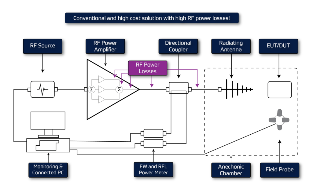
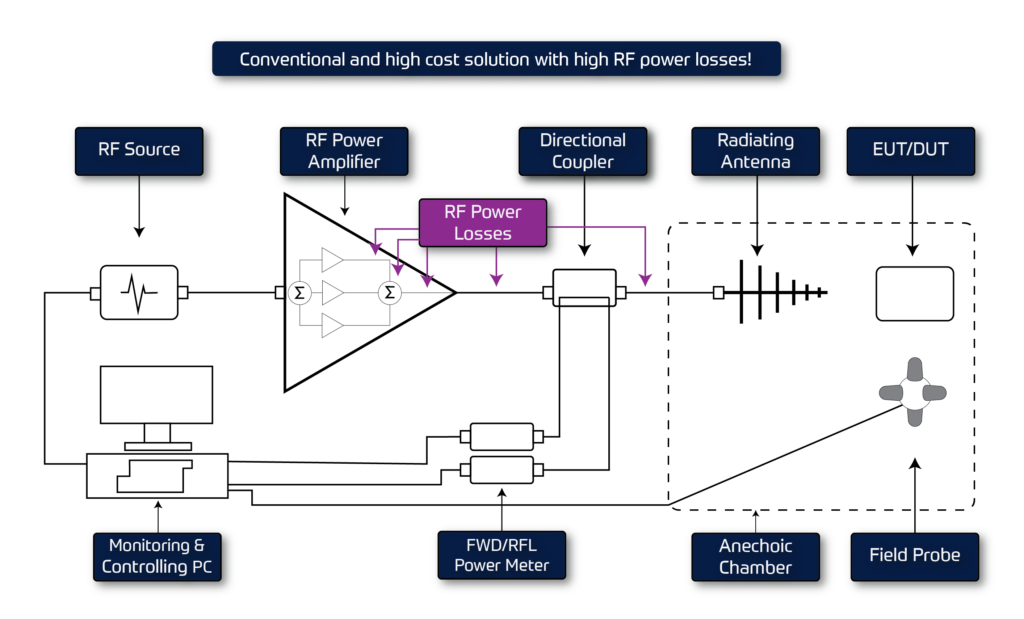
A conventional Chamber and System Setup system is depicted in Figure 1. In a traditional RF Immunity setup, it’s recommended to position the Amplifier-rack (Single or Dual band) and supporting equipment such as signal generator, power meters, couplers, and control PC outside the test chamber. The final field level is influenced by critical items such as coaxial cables and connection joints as listed below:
- From the amplifier output to the input of the Dual Directional Coupler (DDC).
- Between the DDC output and feed through panel on the chamber wall.
- From the chamber feed through panel to the antenna input.
Power losses
The purple coaxial cables play a crucial role in EMC test systems, and it’s important to consider the frequency-dependent losses of cable sections when designing such systems. Typical losses range from 1 to 2 dB, and it’s essential to also factor in the insertion losses of the coaxial connections, which can result in an overall loss of 2.5-3.0 dB. Although having the RF immunity rack inside the test chamber can be a solution to reduce cable length, it’s not compliant with the standard, and losses will still occur. Additionally, when the immunity test rack is inside the chamber, it can impact the measurement, and the test equipment inside the rack must withstand the field levels (self-influence). Another disadvantage of this conventional method is the time-consuming process of moving the setup in and out of the chamber.
Antenna and amplifier considerations
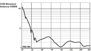
VSWR ratios > 1:6 are frequently encountered in EMC applications. A VSWR of 1:6 implies that 50% of the output power is reflected and returned to the amplifier’s final stage. In the upcoming sections, we’ll discuss some application examples in the 20 to 1000 MHz (and higher) frequency range and how the VSWR impacts amplifier selection.
Electric magnetic field generation below 80 MHz
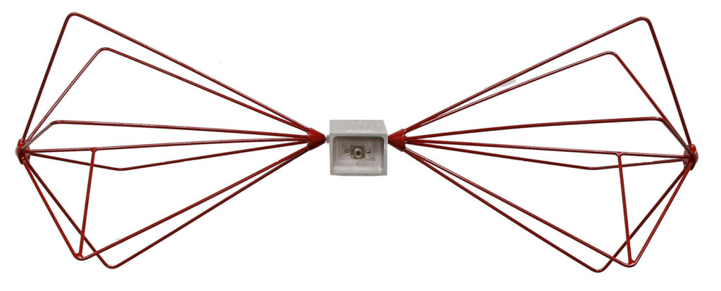
When testing is conducted at low frequencies (between 20 and 80 MHz), high VSWR ratios are commonly encountered. This is because the long wavelengths in this frequency range make it challenging to achieve a compromise between matching, efficiency, and antenna size for compact EMC antennas. Figure 3 illustrates an example of such an antenna, the Biconical antenna. The Biconical antenna and other “small” antennas have designs that compromise on size and are suitable for use in anechoic test rooms.
Higher frequencies | up to 1 GHz
As frequencies increase, the wavelengths become shorter, making the size of antennas closer to their respective wavelengths. Consequently, antennas become a better match to the RF amplifier. Common antenna types used in higher frequency regions include Log Periodic Dipole Arrays (LPDAs), Horns, and Ridged structures, which typically have VSWR ratios well below 1:3.
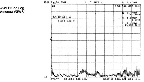
Higher frequencies | 1 GHz and above
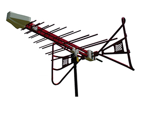
Examples of antennas and their VSWR curves can be seen below. The bent elements in the back shorten the distance between the antenna’s phase center and the DUT, improving efficiency. Figure 5 shows the power vs field graph at 3m for this antenna. LPDA or Horn antennas are the most common types for frequencies above 1 GHz and provide a good 50Ω match to the amplifier’s output.
RF Power considerations 80 – 1000 MHz with an LPDA
Reading graph 5 we can conclude as follows for the lowest frequency, 80 MHz:
- Power to create 10 V/m non-modulated CW 50 Watt CW
- Peak Envelope Power to create 10 V/m + 80% AM = 161.5 Watt PEP* (+ 5.1 dB to the CW power level)
- Average Power with 80% modulation 66 Watt Average ( + 1.2 dB to the CW power level)
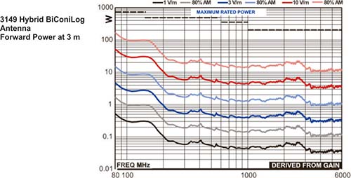
*The definition of PEP power in AM modulated signals is the power-level when the modulation is at its maximum.
CW versus modulated
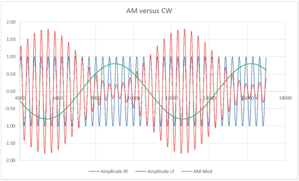
Graph 6 shows the symmetrical AM Modulation envelope to the CW carrier peak voltage. The modulated signal’s average voltage is equivalent to the CW signal’s average voltage. However, signal power is a function of the power of two of the RMS voltage. Therefore, the average power of the AM modulated signal is slightly (1.2 dB) higher than the un-modulated power.
What is needed?
When powering these antennas, 150 Watt amplifiers are common. It’s crucial to consider power reflection and distortion requirements. At 80 MHz, the required forward power is 162 Watts PEP, but we run it at 66 Watts average due to symmetrical modulation.
The VSWR of the antenna results in 50% reflected power, which is 33 Watts. Thus, a 160 Watts Class AB amplifier with a max VSWR of 1:3 is suitable. When designing an EMC immunity system, the two main parameters to consider are:
- The 1 dB compression point, to ensure an undisturbed test signal in the peaks of the modulation
- The VSWR handling capability. This occurs when the antenna VSWR mismatch is high and results in much of the transmitted power to return to the amplifier.
The 1 GHz to 6 GHz band
In the frequency range of 1 to 6 GHz, there are two primary antenna options: Log-Periodic Antennas (LPDAs) and Horn antennas with a gain >12 dBi. The primary distinguishing factor between the two is their respective gain values. While horn antennas have the benefit of a higher gain, they often have a smaller beam, which makes it more complicated to achieve a 1.5 m x 1.5 m uniform field area. Using a horn antenna does not make the EN-61000-4-3 compliance impossible, as above 1 GHz it is allowed to use multiple 50 cm x 50 cm uniform field area windows. A smaller illuminated area is thus still in compliance, but it is less practical, to use a smaller illumination area, as it requires more movement of the antenna, more calibrations, and more bookkeeping of the calibration files to use.
Gain and area of illumination
LPDAs typically have a gain of 7-8 dB, while horn antennas have higher gains that increase with frequency. However, a gain above 12dBi makes EN-61000-4-3 compliance impossible. Higher gain also means smaller illuminated area, making compliance more difficult. The LPDA’s lower gain and larger -6dB angle avoids illumination issues but requires more power to create the required field level. The gain level must be taken into account to comply with the 1.5 * 1.5 meter uniform field area in EN61000-4-3.
VSWR at higher frequencies
The VSWR of these high frequency antennas in general is much lower than 1:3. For this reason Class A is not a real need and Class AB is mostly a good solution.
Selection of the RF power amplifier
Class A or AB amplifier?
The class of amplifier operation is a frequent topic of discussion in EMC immunity testing. Class A amplifiers are commonly recommended to avoid VSWR mismatch affecting the power delivered to the load. It’s important to understand the design criteria and operational limitations of each class before deciding which to use.
Class A amplifier
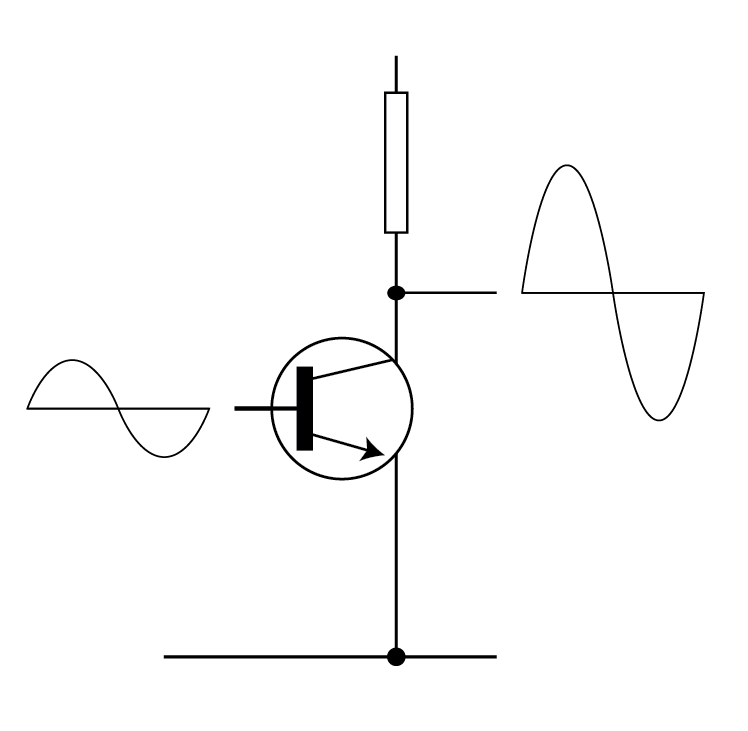
The efficiency of an amplifier, particularly the final stages driving the load, is the primary specification affected by the Class of operation. Figure 7 depicts a basic Class A amplifier, which is known for its linearity. Typically, these amplifiers generate signal currents and voltages that are significantly smaller than the bias values set for them. However, their final stages can only achieve a maximum theoretical efficiency of 50%, although efficiencies ranging from 20% to 30% are common in practice. The single-ended Class A amplifier amplifies the entire signal cycle without significant distortion.
Class B amplifier
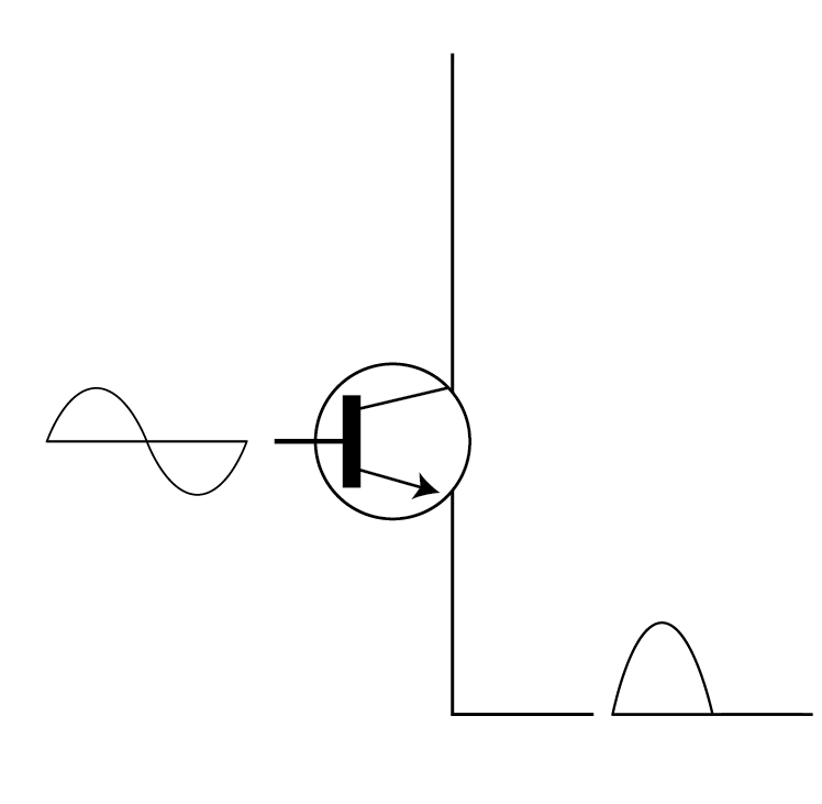
Reducing the bias current to zero will stop the steady-state current through the transistor and reduce power dissipation. In the single-ended Class B amplifier, the input signal is only amplified during its positive cycle, as shown in Figure 8. The input signal must “open” the base-emitter diode of the transistor to allow output current to flow and achieve amplification. This effect greatly improves the efficiency of the amplifier, but signal distortion in the single-ended stage is significant, as only half of the original signal is available at the output.
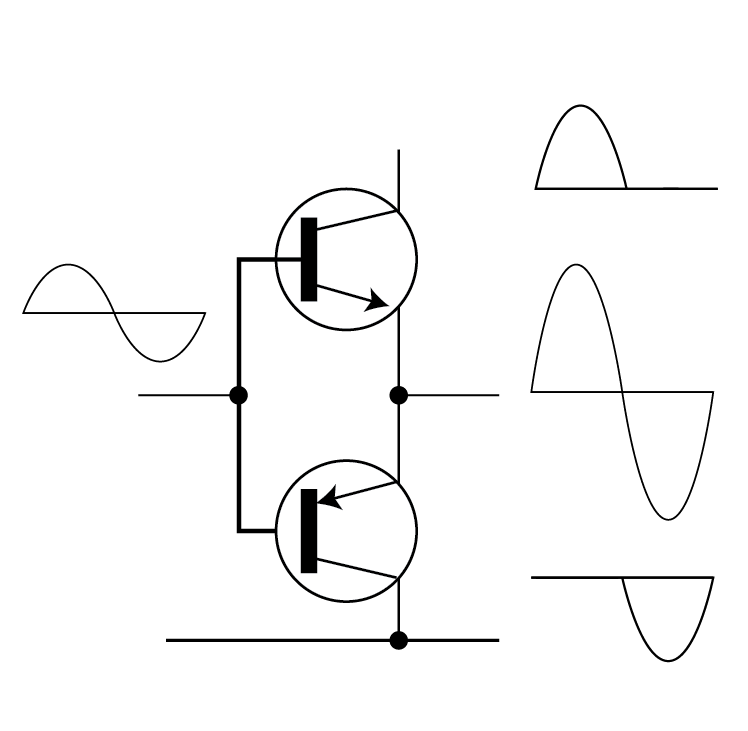
Figure 9 illustrates how a Push-Pull design can improve the output signal by adding the other half of the signal. In this design, two transistors work together, with each one of the pair handling one half of the signal.
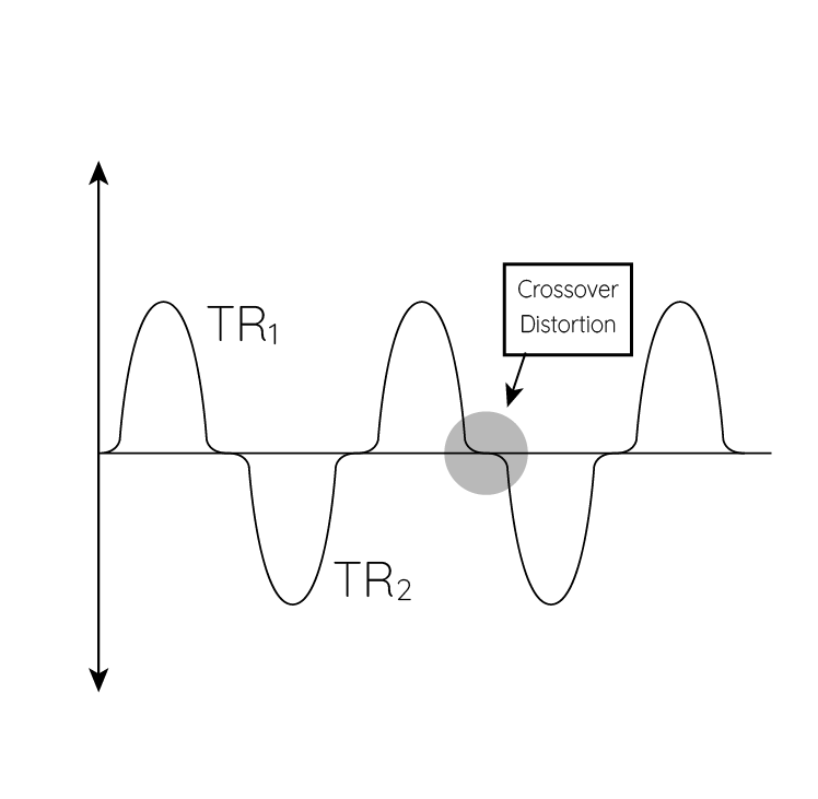
In Class B amplifiers, since the bias current is almost zero, each half of the output signal is not an exact replica of the input signal. The input signal needs to “open” the Base-Emitter junction of each transistor to initiate the signal flow, which results in a waveform as shown in Figure 10. Each transistor begins conducting when the signal voltage crosses the BE diode voltage of around 0.7 Volts to trigger the collector currents. The point where the current flow shifts between the transistors is called the crossover point, and the associated distortion is called the crossover distortion. At low power levels, the crossover distortion has a greater impact on the overall distortion performance of this stage.
Moving to AB
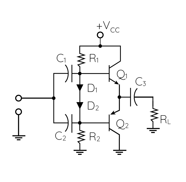
The insertion of a DC voltage that is twice the value of a BE junction between the base inputs of the two transistors, as shown in Figure 11, allows both transistors to conduct and eliminates the undesired behavior around the zero-volt line. This increases the bias current in the final stage, moving from full Class B towards Class A, resulting in a more efficient amplifier known as a Class AB amplifier.
Class A versus Class AB in EMC applications
The topic of whether to use Class A or Class AB amplifiers has sparked a lively debate in the EMC testing world. It’s important to analyze the specific testing application and determine which type of amplifier is truly necessary. In a Class A output stage, the signal current is significantly smaller than the steady state current. This means that even without a signal, the final stage will generate a considerable amount of heat that needs to be dissipated through heat sinking.
Reflected Power
When driving a matched load, the Class A amplifier still exhibits high power dissipation levels in the final stage. Therefore, when there is no load or even a short, the final stage experiences 100% reflection of the output signal’s power, which returns back into the final stage and generates heat. During transistor amplifier design, developers aim to ensure that the total power dissipation of the device falls within the Safe Operating Area (SOA) for reliable and long-term operation. In a Class A solid-state design, the output transistors operate well within their SOA, even with all the reflected power generating additional heat. The SOA considers maximum device voltages, current ratios (power), and thermal power dissipation limits. Refer to figure 12 for the graph.
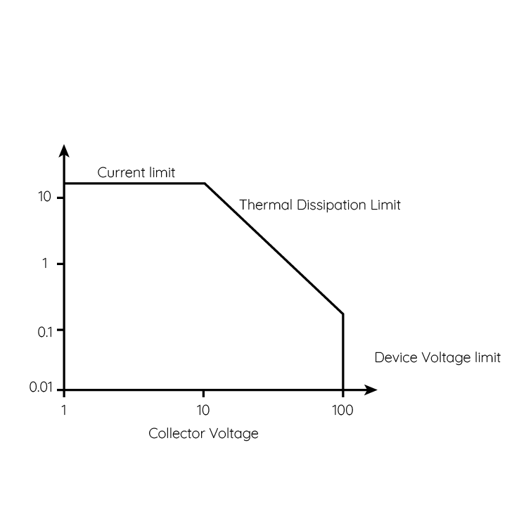
It is evident from figure 12 that the device has constraints on the maximum collector current and voltage. The thermal dissipation limit, which determines the maximum amount of heat a device can generate, is calculated by subtracting the net power supplied to the load from the multiplication of voltage and current.
Differences
In theoretical Class A designs, 50% of the power is lost as heat, whereas in Class AB designs, this loss is reduced to just 12.5%. In Class AB mode, the device has a limited steady state power dissipation with a quiescent current that varies with the drive power. The same transistor used in a Class AB design may deliver less power than in a Class A design due to the thermal constraints under normal load conditions. Additionally, the increased efficiency of Class AB designs results in smaller heat-sink requirements.
The efficiency of the AB type amplifier is best at its high power output levels, which in practice provide up to approximately 60 % practical efficiency. But, what happens if the VSWR of the load increases? Again reflected power from the load returns back into the output devices and is converted in additional heat that can increase the device temperature beyond the SOA curve. When protection measures are not in place, the device will get damaged due to this extra heat. For this reason, class AB amplifiers have a VSWR protection system that lowers the drive to the final stage and reduces the (average) power that must be dissipated.
dB compression point
When the load has good VSWR performance, the differences in compression characteristics between Class A and AB are not significant. Therefore, the 1dB compression point performance is quite comparable between these two classes.
The RadiField® – Electric Field Generator (Triple A)
With the RadiField Triple A (AAA stands for Active Antenna Array) Raditeq sets a complete new standard for immunity testing. RadiField Triple A offers:
- A simplified system approach
- Guaranteed EM field level
- High level of integration
- No loss of expensive RF power
- Low cost of ownership
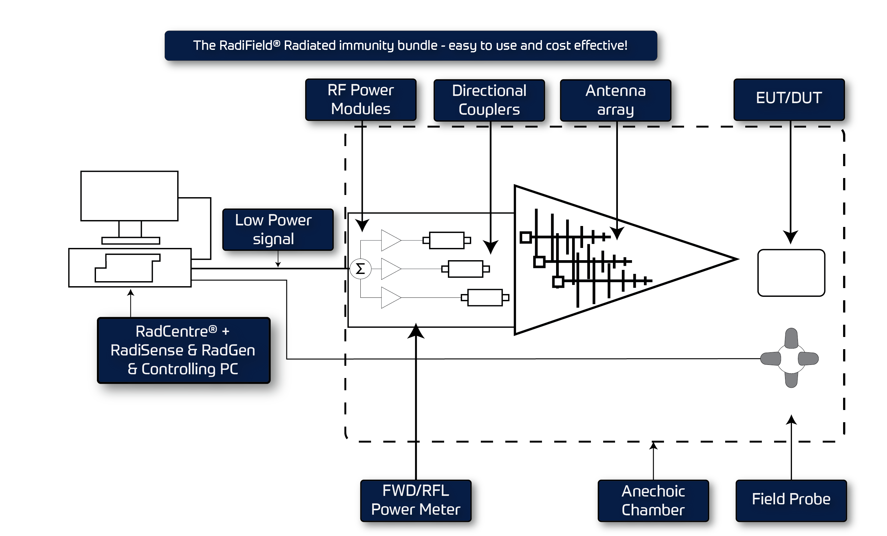
The two setups in Figure 13 show that the complexity isn’t necessary in the case if the RadiField solution (see Figure 14). The system is build up with a RadiCentre® modular system. In the RadiCentre® the following modules are inserted for this application:
- RadiGen® 6 GHz Signal Generator
- RadiSense® 10 GHz Field Probe Laser card
- RadiField® Power Supply and Control Card
This system uses just two coaxial cables. Only one coaxial cable runs from the RadiCentre® RadiField power supply card to the RadiField Triple A carrying:
- Power
- Control / Communication
- Driving RF signal
The RadiGen® output is connected to the RF input of the RadiField® power supply card via a second cable. A Bias-Tee on the card combines DC power, control signals, and RF drive, and all cable losses are eliminated. The RF power is directly fed into the antenna and converted into an electromagnetic field. In a conventional setup, low-loss coaxial cables are necessary to transport the RF power generated by the system to the antenna located several meters away to ensure that the majority of the power is transmitted without loss.
Reducing Complexity of the System
When comparing the traditional setup of an RF immunity test system with the RadiField Triple A, it is evident that the RadiField Triple A provides a solution to reduce both space and costs due to its high level of integration.
The conventional approach
Looking to the basic setup of a conventional system, generally the following system components can be recognized:
- Signal Generator
- RF Power Amplifier(s), single or dual-band
- Dual Directional Coupler(s), one or more bands
- 2 RF power meters (forward and reflected power)
- RF Switches (not needed with a single band amplifier)
Next to the system components in the single band solution, 5 coaxial, and at least 4 control cables are needed. When a Single Band amplifier is not available, the complexity drastically increases to 12 coaxial cables and 5 control cables in case of the Dual Band approach.
Minimum installation time
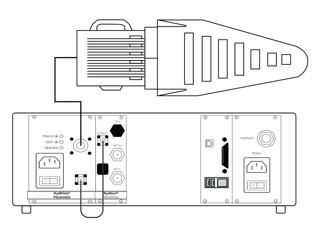
The RadiField’s design allows for a quick and easy installation process for the user. The RadiCentre®, which includes a Signal Generator, RadiField Card, and Laser Driven Field Probe system, is located in the engineer’s control room. With only two coaxial cables needed (from the RadiCentre® to the anechoic chamber’s entry panel and from the entry panel to the RadiField), the generation of an EM field can begin swiftly.
Three Meter Equivalent (TME) field
The RadiField makes it easier than ever before to determine and define the required field level. A new parameter called the Three Meter Equivalent (TME) allows for simple recalculation of field strengths at different distances relative to the value at 3 meters. The formula used to recalculate fields at different distances is:
3 * TME / d
Thus given a system with a TME of 10 V/m, an easy recalculation, shows that this system will generate:
- 10 V/m * 3 / 10 V equals 3.0 V/m @ 10 meters
- 10 V/m * 3 / 1 V equals 30.0 V/m @ 1 meter.
No more worry about amplifier power, antenna gain and gain calibrations at various distances, cable losses versus frequency etc. Just establish your required field level, distance and frequency range, and select the RadiField that covers your needs for the required test distance and field level.
| Model | Frequency | 1m | 3m | 10m |
| RFS2006A | 800 MHz – 6 GHz | 9 V/m | 3 V/m | 0.9 V/m |
| RFS2006B | 800 MHz – 6 GHz | 30 V/m | 10 V/m | 3 V/m |
Accuracy and reliability
During the Radiated Immunity test, the operator positions the Device Under Test (DUT) in a pre-calibrated uniform field using a field-probe placed in 16 equally spaced positions within the uniform area. After the calibration is complete, the operator removes the field probe and uses the pre-calibrated values to illuminate the DUT during the test.
The field calibration process involves recording the relationships between the measured field levels and the power levels on the output ports of the directional couplers placed behind the RF power amplifiers. When executing the test and after removing the field probe from the chamber, the control software uses the directional coupler’s forward and reflected power data to replay the power levels.
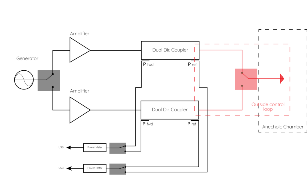
The test does not measure or correct for changes in signal attenuation resulting from variations in cable loss, switch-loss, and connector loss in the cables highlighted in red in Figure 16, despite measuring all components from the signal generator to the directional couplers.
Although the operator may believe that the test is running correctly, there is no guarantee that the test is the same as during the calibration run. The design of the RadiField eliminates all sources of errors by integrating the radiating antennas, RF power amplifiers, and couplers into a single system.
Electric Magnetic Field Combining & Cost of Ownership
Finally, the RadiField offers an attractive total cost of ownership compared to traditional setups. A comparison table has been created to compare the RadiField with other combinations of amplifiers and antennas. The unit’s base price is approximately 50% lower than conventional setups, and maintenance costs are reduced due to less wear and tear and no need for separate calibration of cable losses, antenna gain, coupler, and RF power meters. This doesn’t even take into account the time required for installation and re-installation (e.g. antenna switch) and potential errors due to the complexity of conventional systems are difficult to quantify. For the comparison, similar setups are defined as follows:
Conventional Setup contains:
- Signal generator
- Power amplifier
- Coupler
- Forward power meter
- Reflected power meter
- Antenna
- Field Sensor
- Cables and connectors (6 sets)
RadiField Electric Field generator setup contains:
- RadiCentre including
- RadiSupply
- RadiGen Signal generator
- RadiSense Field Sensor
- RadiField Triple A
- Cables and connectors (2 sets)
List of Abbreviations
TME – Three meter equivalent
SOA – Safe Operating Area
VSWR – Voltage Standing Wave Ratio
DUT – Device under Test
DDC – Dual Directional Coupler
EM – Electro Magnetic
LPDA – Log Periodic Dipole Array
PEP – Peak Envelope Power
Triple A – Active Antenna Array
Accredited Test Laboratory Results.
We have tested the RadiField in anechoic test chambers of KIWA DARE Services to obtain a validation of this test system towards the proposed field levels and the uniformity of the illuminated area. The results of this test can be found in the downloadable PDF.